Simulated annealing

< Simulated annealing이란? >

Kirkpatrick AI 가 1983년에 particle system의 thermo dynamic에서 영감을 받아 만든 "담금질 기법"입니다.

높은 온도에서는 금속의 원자들이 액체 상태이기 때문에 더 자유롭게 움직이고, 쿨링(온도를 낮추게 되면) 다시 Solid고체 상태로 돌아옵니다.

냉각이 빠르면 원자는 한 상태에서 응고가 되기에 생성 된 합금은 구조가 불규칙하고 고 에너지를 갖게 되죠.

반면, 냉각이 느리면(Annealing) 원자가 스스로 재구성되고 생성된 합금은 완벽한 결정 구조와 최소 에너지를 갖게 됩니다.

(* basse : 낮은, élevée :, 높은)

 

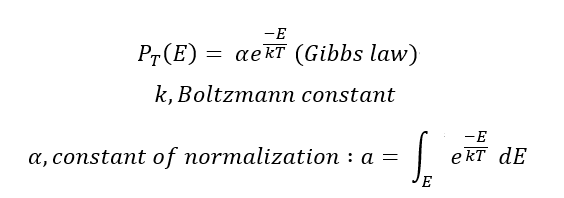
1)Energy level (에너지 레벨)

- 만약 System energy level E가 원자의 배열에 의존적이라면,

특정 온도 T에서 확률 Pt(E)인 System Energy E는 아래와 같게 됩니다.

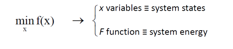
2)Minimize 문제에 적용

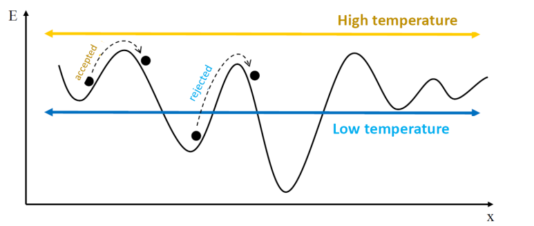
이 Simulated annealing방법을 이용해 Global minimum이나 Global maximum을 찾을 수 있습니다.

예시로 Minimize문제를 들겠습니다. Global minimum을 찾는 게 목표일 때, 원자는 높은 온도에서 더 높은 hill로 Jump를 하게 되고, 낮은 온도에서는 hill에서 내려오게 됩니다.

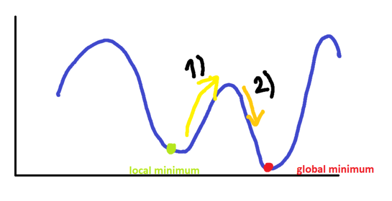
아래 그림과 같이 Local minimum과 Gloabal minimum이 있다고 할 때, (y축은 함수값이라고 합시다.)

​

1)의 경우 함수값 f(x) < f(x+1)

 그 다음 x+1의 함수값이 더 크게 되는데, 이 경우 목표는 최소값을 찾는 거기에 사실상 함수값이 커지면 좋지 않은 move입니다.

그치만, 우리는 Randomly하게 이 과정을 수락하며 global minimum을 찾기 위해 나아가는거죠.

​

2)의 경우 함수값 f(x) > f(x+1)

이 경우 그 다음 x+1의 함수값이 현재 지점 x의 함수값보다 작으므로 이 과정은 100 퍼센트 허용합니다.

 

3)Metropolis Algorithm (1953)

아까 위에서 봤던 1)의 경우를 randomly하게 수락한다고 했죠?

Metropolis Algorithm에 기초하여 새로운 State를 받아들이게 됩니다.

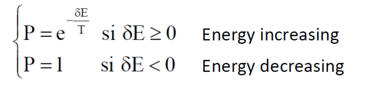
높은 온도에서는 Accept할 확률이 커지게 됩니다.

여기서 우리는 T를 함수값 f(x) / System energy 로 간주합니다.

​

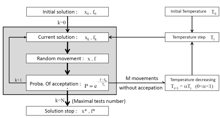
4)Simulated Annealing Alogirhtm

대략적인 Algorithm block diagram입니다.

 

위의 알고리즘을 MATLAB으로 구현하려면 어떻게 할까요?

1) Initial point x0 , f0(함수값) 을 잡습니다. 초기 온도 T0는 충분히 높은 값으로 잡고 Iteration n 도 정합니다.

종료 crieterion epsilon값도 정합니다.

​

2) x의 randomly한 Neighbors값 x(t+1) = N x(t)를 계산합니다.

​

3) If delta(E) = E(x(t+1)) - E(x(t)) < 0, 이라면 t = t+1으로 세팅해줍니다.

Else 그 외에는 random number r을 범위(0,1)에서 생성합니다.

If r<= exp(-delta(E)/T)라면 , t = t+2로 세팅합니다.

Else 그 외에는 다시 Step2로 갑니다.

**여기서 delta(E)는 에너지 레벨 차이, 즉 함수값의 차이입니다.

​

4) If abs(x(t+1)-x(t)) < epsilon 이고 T가 작은 온도라면 종료합니다.

Else if (t mod n)=0 이라면 다시 step2로 이동합니다. (더 낮은 T 값을 찾기 위해서..)

 

 

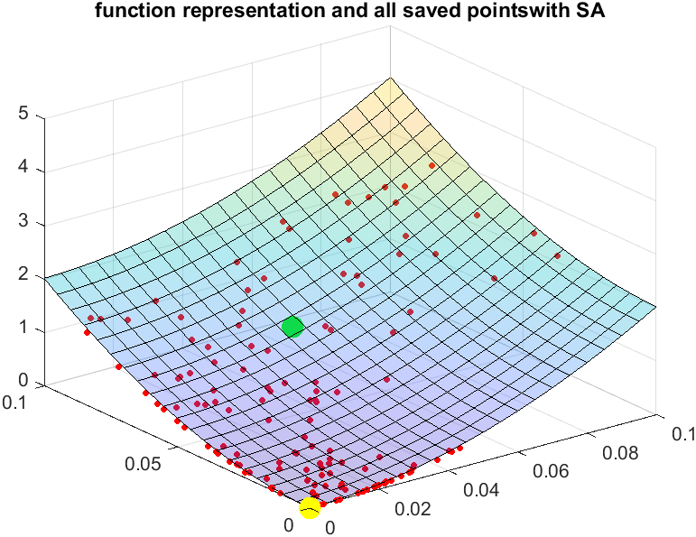
아래는 실제 직접 구현한 Matlab code와 결과 사진 입니다.

interval x[0,0.1] and y[0,0.1]에서 찾은 최소값은 0,0 입니다.

 

 

 

All point with Simulated annealing method

 

---------------------------------
our last point saved is
X = 2×1
0
0
with a fitness value =
ans = 0
---------------------------------

 

Simulated Annealing simulation을 위해서는 Cooling down coefficient와 Iteration number을 잘 설정해주어야 합니다.

Particle Swarm method에 비해 Iteration number가 많이 필요하며, Cooling down coefficient가 너무 크다면 Temperature가 너무 느리게 감소하기 때문에 bad points를 Accept할 확률이 높아집니다.

 

clear all;
close all;
clc;

syms x y % we made symbolic variable x and y
fun = 20 + x^2 + y^2 - 10*(cos(2*pi*x) + cos(2*pi*y));
alpha = 1;
g=alpha * fun

figure(1)
[x1, y1] = meshgrid(0:0.005:0.1); 
surf(x1, y1, alpha*(20+ x1^2 + y1^2 - 10*(cos(2*pi*x1) + cos(2*pi*y1))),'FaceAlpha',0.3); %we plot function to see what it looks like


%%%%%%%%%%%%%%%%%%%%%%%%%%%% variables %%%%%%%%%%%%%%%
Xres = [0 0.1];
Yres = [0 0.1];

ini_pt = 4; %to calculate initial temperature
K = 1 ; %boltzmann constant

Max_it = 300;
cooldwn_cycles = 5; % every X points not accepted we cool down
coeff_cooldwn = 0.9; %everytime we cooldown we multiplicaqte temp by coeff
cldwn = 0;

iteration =1;
fitness_v=[];
T_v=[];
%%%%%%%%%%%%%% calculating initial temperature %%%%%%%%%%%%


R1 = (1/10)*rand(1,ini_pt);
R2 = (1/10)*rand(1,ini_pt);

FITNESS = subs(g,{x y},{R1 R2});
T = sum(FITNESS)/ini_pt; %initial temperature

%%%%%%%%%%%%%%%%%% initial point %%%%%%%%%%%%%%%%%%%%%%%%%

X(1,1) = (1/10)*rand(1);
X(2,1) = (1/10)*rand(1);

FITNESS = subs(g,{x y},{X(1,1) X(2,1)});
iteration =1;
hold on;
plot3(X(1,1), X(2,1), FITNESS,'.g','markersize',40);
title('function representation and all saved pointswith SA')
fitness_v=[fitness_v FITNESS];
T_v=[T_v T];
%%%%%%%%%%%%%%%%%%% Generating new design point %%%%%%%%%%

    borders_x = (max(Xres)-min(Xres))/4;
    borders_y = (max(Yres)-min(Yres))/4; 

while (iteration < Max_it)
    U1 = rand(1);
    U2 = rand(1);
        
    X_temp(1,1) = X(1,1)-borders_x + U1*(X(1,1)+borders_x-(X(1,1)-borders_x));
    X_temp(2,1) = X(2,1)-borders_y + U2*(X(2,1)+borders_y-(X(2,1)-borders_y));
   
    if X_temp(1,1) > max(Xres) || X_temp(1,1) < min(Xres)
        if X_temp(1,1) > max(Xres)
            X_temp(1,1) = max(Xres);
        else
            X_temp(1,1) = min(Xres);
        end
    end
       
    if X_temp(2,1) > max(Yres) || X_temp(2,1) < min(Yres)
        if X_temp(2,1) > max(Yres)
            X_temp(2,1) = max(Yres);
        else
            X_temp(2,1) = min(Yres);
        end
    end
    
    New_fit = subs(g,{x y},{X_temp(1,1) X_temp(2,1)});
    
    delta_g = New_fit-FITNESS ;
    
    if (delta_g<0)
        X=X_temp;
        FITNESS = New_fit;
         hold on;
         plot3(X(1,1), X(2,1), FITNESS,'.r','markersize',10);
         fitness_v=[fitness_v FITNESS];
         T_v=[T_v T];
    else
        %%%%%%%%%%%%%%%%% METROPOLIS CRITERIA %%%%%%%%%%%%%%%%%%%%%%%%%%%
        R_metro = rand(1);
        P_X_temp = exp(-delta_g/(K*T));
        
        if (R_metro<P_X_temp)
        X=X_temp;
        FITNESS = New_fit;
        hold on;
        plot3(X(1,1), X(2,1), FITNESS,'.r','markersize',10);
        
        fitness_v=[fitness_v FITNESS]; %%%%% data analysis
        T_v=[T_v T];%%%%% data analysis
        
        else                                %WE DONT ACCEPT THE POINT
            cldwn=cldwn+1;                  %WE DECREASE TEMPERATURE
            if (cldwn == cooldwn_cycles)    %IF WE REACH A CERTAIN CYCLE OF NON ACCEPTATION
                T=coeff_cooldwn*T ;         %WE DEACRESE THE TEMPERATURE
                cldwn=0;
            end
        end
    end
    iteration=iteration+1;
end

hold on;
plot3(X(1,1), X(2,1), FITNESS,'.y','markersize',40);

figure(2)
t=0:length(fitness_v)-1;
plot(t,fitness_v,t,T_v)
title('evolution of fitness and temperature');
legend('Fitness','Temperature');

disp('---------------------------------')
disp('our last point saved is')
X
disp('with a fitness value =')
double(FITNESS)

 

 

출처: elgar328.tistory.com/11 티스토리 소스코드 입력하기